Parametric simulation

Talks

• Software meeting 2018-06-29, Friday, File:Sctau papas v2 20180629.pdf

About papas, heppy et cetra

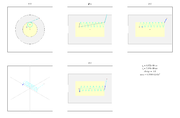
Particle propagation is done by geometry calculation. To valid the calculation several different cases were plotted.

Helix.

Configure detector parameters

The detector parameters can be changed via the a configuration file CTauPapas.cfg placed in the main papas simulation folder. The file has a simple structure --- one parameter and its value(s) per line. A parameter's name and value(s) should be separated by spaces. Empty lines and lines beginning with # are ignored.

In the example below the parameter at the first line is one number, while the parameter at the second line is an array.

ecal_emin_barrel 0.05

ecal_eres 1.34e-2 0.066e-2 0 0.82e-2

The parameters can be given in any order.

How to run papas

Copy a directory with papas on stark the machine and go to this directory.

cd

cp -rf ~razuvaev/myheppy .

cd myheppy

There are a directory output for output files, detector configuration file CTauPapas.cfg, file ctau_input_sim.txt with a path to the file with primary generator events, and the folder heppy with heppy code itself. Let's go into it and tune environment.

cd heppy

source init.sh

Now it is time to run papas. You may be asked a question because the output directory is not empty. So just input y or clean the folder.

cd test

./heppy_loop.py ../../output/ ctau_cfg1.py

When papas simulation has been done one need to present papas output to a suitable form and also add initial generator information.

cd ../../

./txt2rtee.py

The output root tree is available in the file myheppy/output/txt2tree.root.

Output tree

The output tree contains branches which can be divided in several groups:

• reconstructed particle parameters;
• generated particle parameters;
• generated vertices;
• connection between reconstructed particles, generated particles and generated vertices.

The table below presents branches and description of their content.

Name	Type	Length	Description
Reconstructed particles
n	int	1	The number of reconstructed particles.
px	float []	n	The reconstructed particle momentum: x coordinate.
py	float []	n	The reconstructed particle momentum: y coordinate.
pz	float []	n	The reconstructed particle momentum: z coordinate.
Generated particles
n0	int	1	The number of generated particles.
px0	float []	n0	The generated particle momentum: x coordinate.
py0	float []	n0	The generated particle momentum: y coordinate.
pz0	float []	n0	The generated particle momentum: z coordinate.
Generated vertices
nv0	int	1	The number of generated vertices.
vx0	float []	nv0	The generated vertex: x coordinate.
vy0	float []	nv0	The generated vertex: y coordinate.
vz0	float []	nv0	The generated vertex: z coordinate.
Links
recgen	int []	n	Transform a reconstructed particle index to the generated particle index.
genver	int []	n0	Transform a generated particle index to the generated vertex index.

Analysis example

Here a short analysis example of $D^0 \to K_S^0 \pi^+ \pi^-$ is presented. The things are performed with PyROOT.

The data a taken from the available exclusive sample.

The code can be taken from github [1] or find at the stark cluster: /home/razuvaev/myheppy/search_dkspipi.py.

• 

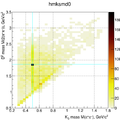
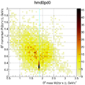
  $K_S^0$ mass vs $D^0$ mass.

• 

  $D^0$ mass vs its momentum.